This post follows up from my recent one entitled ‘AWS Serverless Analytics: The Promise…’ in which I described the value proposition for serverless analytics.

In today’s update, I have a database hosted in Amazon Aurora, which we will crawl and automatically catalog with AWS Glue, load it into an S3 data lake using Glue, and then query it in Amazon Athena, all without the work of instantiating any server hardware, operating systems, or configuring applications for database management, ETL, or cataloging.

Tables of Interest from an Operational Database

For our demo, we will be working with the six tables shown in the E/R diagram below, a subset of an OLTP movie rental database.  For visual clarity, child tables are depicted below parent tables.  To summarize the relationships, film and category have their many-to-many relationship controlled by the associative film_category table.  One customer may purchase multiple rentals.  On one rental purchase, one customer might make multiple payments.  

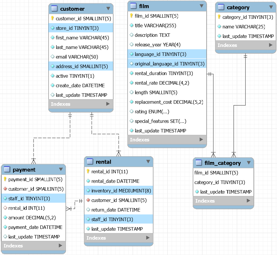
The above diagram is from the MySQL Workbench UI on my desktop, but the database and it’s data is stored as a (serverless) Aurora MySQL database in Amazon RDS.  Aurora also supports serverless PostgreSQL.  

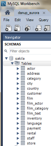
For future reference, although our source database, as the below screenshot shows, has additional tables (and some views), I will limit our demo to the six tables shown in the diagram above.  

Amazon’s AWS Console:

As this is our first look into the AWS Console, understand that doing so yourself requires you to create an AWS account (the free tier makes it easy to start and the Billing Dashboard makes it easy to understand if and when you do incur charges and how much.  If you prefer to simply read this blog, I have pasted sufficient screenshots to give you a visual reference to what I’m doing and where. 

From my own usage of AWS Console, including file uploads and processing in RDS, Glue, Athena, and Quicksight, I’m finding monthly charges to be $30 to $60, and each or all of these services are easy to turn off when not needed.  For just browsing along with me, even though you must enter a credit card to create a free account, your changes will be near zero until you actually process data.  In this demo, you will not need to, but I will show you how to view your actual and projected AWS charges.

AWS Console Fundamentals

Not to provide in-depth coverage of what is on the AWS console, I will just provide some hints if it is unfamiliar.

• Login / Signup: https://aws.amazon.com/.  In the top right is the sign-in / sign-up prompt. 
• Once logged into the AWS Console, click the Services button on the left side of console header bar, and referring to the screenshot below, note…
  • All services are categorized for your convenience
  • Because you won’t immediately remember the services in each of these categories, start out simply by  searching on your item.  For instance, search on ‘Glue’.
  • Note, however, the location of the Analytic category, in which links to most of the products we will demo are location.
  • As you click around, your recent services clicks will accumulate in the left pane for easy re-use.
  • Because you will eventually find yourself clicking back and forth between related consoles (in our case, S3, Glue, Athena, and Quicksight), when you do find them under services, I recommend that you make a habit to ‘Open in New Tab’, so you can navigate between multiple services fast. 
  • Lastly, in the aforementioned header bar, click the push-pin icon, find services you know you’ll want handy for re-use, and drag them up to the header bar to customize your AWS Console.
  • With that, we will jump into the individual consoles.

AWS Services by Category

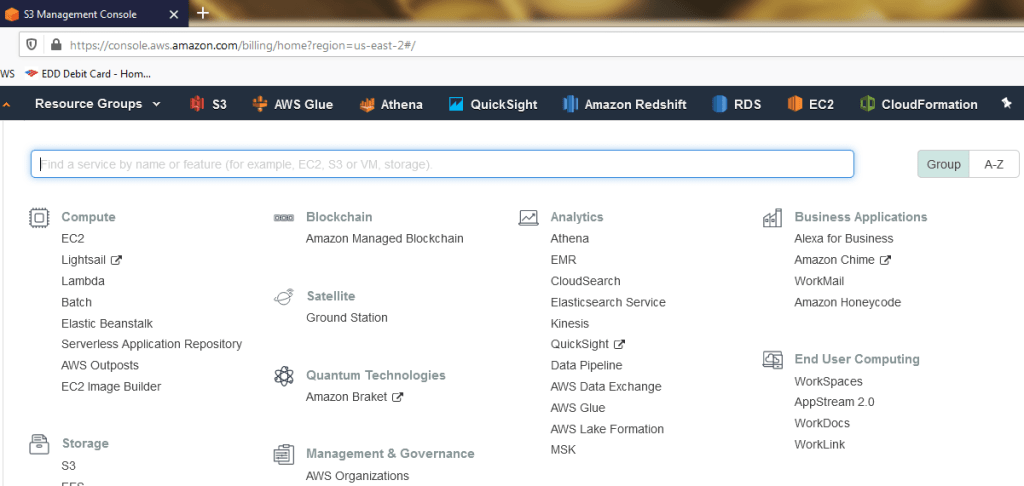
To see the screenshot below, from the AWS Main Console, click the Services tab, then note everything under Analytics, plus Storage / S3.

_____________________________________________________

Aurora – Amazon Web Services’ Serverless Option in Relational Database Services (RDS)

General Discussion on Aurora:

In Amazon RDS, a list of popular database systems can be instantiated to run on EC2 instances with a variety of capabilities.  Aurora, the RDS service we will use, is Amazon RDS’s version of a serverless PostGreSQL or MySQL database. Being serverless, it removes the work of instantiating, backing up, patching, upgrading and supporting actual database servers, the hardware, the OS and the database applications.

• Because of Aurora’s separation of logging, storage and caching from the relational engine, it is purpose built to…
  • Minimizes table-locking contention
  • Guarantee that a database instance re-start will not require re-warming of cached data

Aurora also provides…

• Fault tolerance, by default, across Availability Zones (AZ’s) and optionally, across Regions, too.
• Continual incremental data backups
• Quickly scaling up and down based on changes in computing or data volume without interfering with activity from ongoing connections.
• Being a managed (serverless) service, Aurora charges are usage-based.  Aurora databases that will not be needed for a time can be easily backed up to S3, at which time the Aurora Instance can be terminated and the RDS charges stop.  If and when needed later, it can be re-instantiated and the data restored.

Summary Recap of Our Configurations in Aurora:

In the RDS Console, during our MySQL database instance creation, we are prompted to name the instance, specify ‘Serverless’, select region(s), input master credentials, connectivity to a specific Virtual Private Cloud (VPC, and the server’s capacity.  For the serverless (Aurora) architecture, we choose minimum and maximum CPU/RAM capacity.  The available range is from a minimum of 2 vCPU’s and a minimum 2 GB RAM up to 96 vCPU’s and 488 GB RAM, with many choices in between, so that the system can scale up and back down as we determine in order to maintain a margin of available capacity. 

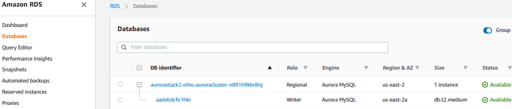
Not much else to do here.  Just note that the DB Instance is an Aurora MySQL, is in Ohio (us-east-2), and is now available.

_________________________________________________

I think of AWS Glue as a data engineering suite; a combination data crawler, one-stop queryable data catalog, and scalable ETL engine all in one.  Although serverless by default, VPC endpoints, which instantiate development and test environments (machines), can be configured within Glue to satisfy a team’s need to write and test Glue scripts. So, with a dev and/or test environment, Glue is no longer 100% serverless, and these endpoints are billable the entire time they are instantiated.

The plan here is to catalog the tables in the above ER Diagram and then load them into S3. Our first step is to run an AWS Glue Crawler simply to catalog this data, storing it into the Glue Data Catalog, to which we will then connect, setup and run a Glue ETL Job. 

General Discussion on AWS Glue: 

Before we set up the crawler, let’s talk about Glue.  The Glue Data Catalog is built from the Apache Hive Metastore for Presto.  It stores no actual data records, but does store all of the metadata:  essentially the paths, names, and properties of databases, tables, and fields, such that not only Glue ETL jobs, but also the RedShift Spectrum and Athena query engines can query the Glue Catalog itself and pull data directly from the S3 data lake that Glue has catalogued.

The diagram below illustrates the general architecture of Glue Crawlers, Data Catalog and ETL

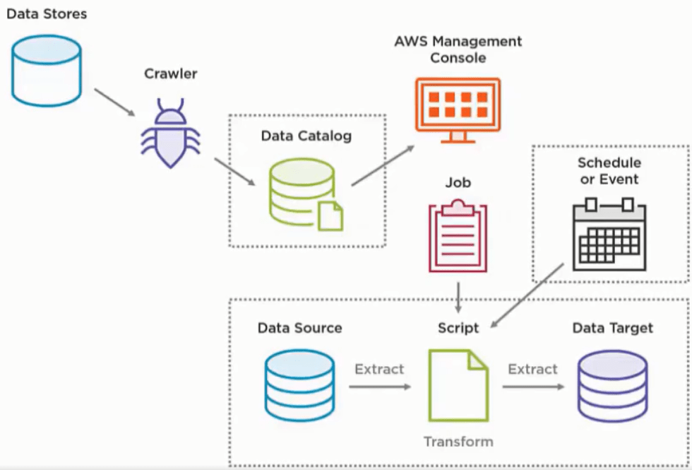
Referring to the above screenshot, here is an example:

1. Crawl a data store to classify the data format and store it’s metadata and path in the data catalog
2. Build one or more ETL Jobs, orchestrate any job dependencies using Glue Triggers within a Glue Workflow, to land the data, perhaps un-transformed initially, as files in S3, the data target.
3. Either schedule the workflow or set it to run based on an event, kicked off via a Lambda function that detects, for example, a new file arriving in an S3 folder.
4. Crawl the new S3 files to catalog them.
5. Build more ETL to transform the data, as needed
6. Crawl the transformed files to catalog them.
7. Setup a post-ETL crawler to deal with schema changes in the catalog.

With that, the data is ready in S3 and queryable via the Glue Data Catalog.

Hands On Glue (-:

The Glue Console looks like this:

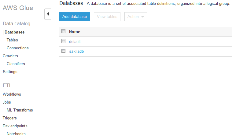
While here, let’s note a few items above on the left margin.  In Glue, a database is simply a grouping of tables that share the same connection.  A Crawler selects from a hierarchised list of Classifiers, each of which attempt to automatically parse different major types of data.  Out-of-the-box, Glue has built-in Classifiers for MySQL, PostGreSQL, SQL Server, Parquet, ORC, JSON, CSV, and a few others, and custom classifiers can also be built.

To build a Crawler, we first need a connection, one of which is shown here.

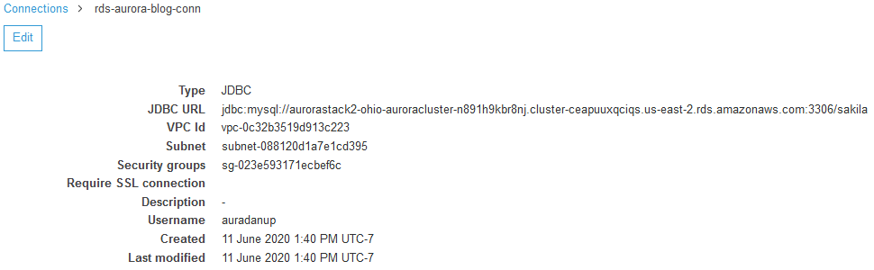
This is a JDBC connection, but Glue also connects directly to S3 and DynamoDB. Notice that the URL includes the region, RDS host-endpoint, port (3306 is the MySQL default), and database name.  Also specified is the VPC, subnet, and security group under which the named user is granted access to this data store.  On clicking Edit (or Add), the above items are all entered with a UI with convenient prompts and fields for copy/pasting. As always with AWS, you will want multiple consoles open in tabs.

With the available connection, we build a crawler and, once built, it will look something like this.

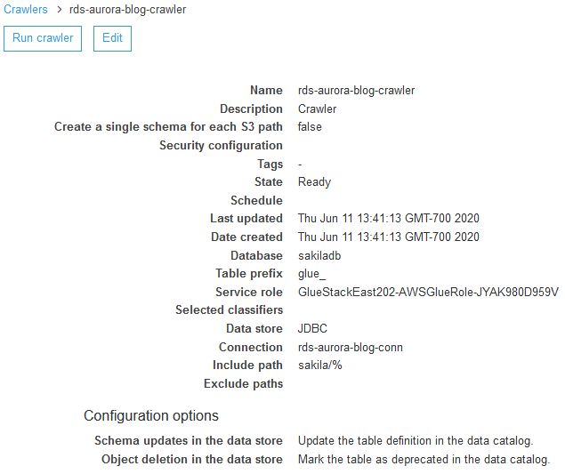
Note the following:

• Although the above Crawler crawls only one data store, a crawler can crawl multiple ones, sensible if they are very similar.
• ‘Create a single schema for each S3 path: I leave it unchecked (the default).  When we run a crawler against S3, instead of against Aurora-MySQL here, we will want to first have planned our S3 folder structure as to whether or not Glue can infer a single schema, based on similar metadata, across separate folders or not.
• Table prefix (pre-pend):  This is helpful in that, depending on the source data structure (…databasename.tablename, or perhaps S3FolderName.SubFolderName.FileName.PartitionName), we may want to pre-pend a crawler-specific prefix to objects going into the data catalog, which importantly will otherwise be catalogued with the same object name as in the data source. 
  • Side-bar: Remember, we’re not doing ETL yet, just crawling a data store to build a catalog for subsequent usage.  Also, when we do the ETL to load the data lake with raw, untransformed data, we will also avoid renaming fields in that stage.  What we will want to do at that point, is to run a new crawler to catalog the data now in the data lake, and then do additional ETL in which we transform the data, possibly renaming tables or fields, load it into a presentation layer, and then once again catalog it so that, for example, Athena or Redshift Spectrum can identify and query the presentation layer data.

• The Service role specifies the level of access granted to this crawler to the data source.
• Classifiers: During a crawl, the data stores object formats are evaluated by a sequence of built-in classifiers — and custom classifiers that you can build — to determine to which class of data formats of them the data set belongs, whether it is CSV, JSON, Parquet, any number of RDBMS platforms, or something else.
  • Glue Classifier documentation is available here.
• Include Path:  Specifies the scope of tables in the database (in MySQL, [ YourDBName/%  ] indicates all tables)

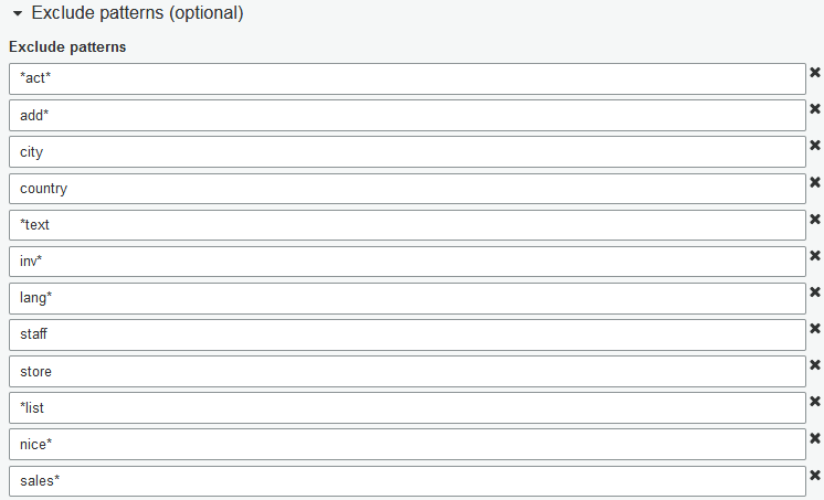
Exclude Patterns: 

Within a specified Include Path, Exclude Patterns, while optional, are actually the fundamental way we specify objects not to be catalogued. In an RDBMS data store to be crawled, some views may be worth cataloguing, so understand that Glue catalogs a view as if it is a table. So, to the extent that a view is not desired for cataloguing, Exclude Patterns are used to exclude it according to it’s name or naming pattern. See AWS Glue documentation (scrolling down to ‘Include and Exclude Patterns’) for additional guidance. Exclude patterns can also articulate an intended S3 folder structure path.

Exclude patterns are simple, especially for relational tables.  In the screenshot below, I use the patterns shown to limit our crawler to just the tables in our ER diagram.  Comparing this screenshot to the above screenshot of all tables in the database, you will note that my first entry, *act*, excludes all tables with a name containing the string ‘act’ with any number of characters before or after.  Note also that, unless individual views name-patterns are specified in Exclude Patterns, then they, too, will be catalogued. 

Crawler Output Configuration 

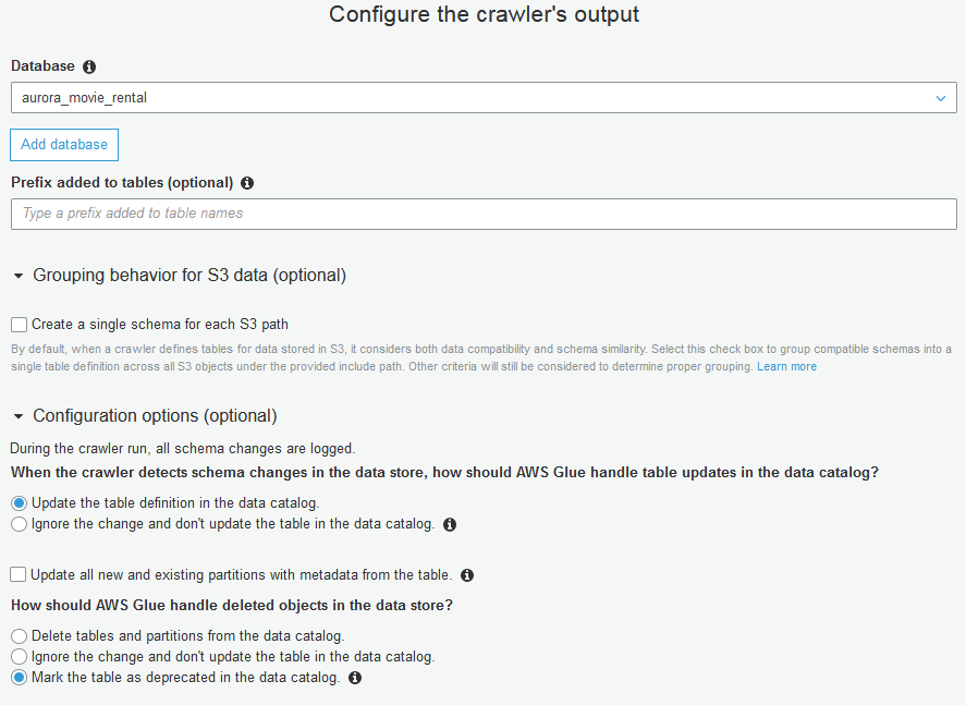
Referring to the above screenshot.

• Database: Although we may simply use the name of the source data store for this, we can also specify another name for these tables going into the data catalog, as I’ve done here.
• Prefix (optional): 
  • Before considering whether to use this optional field to pre-pend table names, note that all tables from an RDBMS data store will already (always) be pre-pended with database name.
  • As appropriate, what is entered here is pre-pended to each incoming object in this order: (prefix_database_table).  Examples of reasonable prefixes might be:  (schema_name, stage, etl, presentation, aggregate, presto, athena, etc).  Not needed here, so I will skip it.
• Create Single Schema for each S3 Path:  Allow the crawler’s (built-in or your custom) classifiers to scan multiple S3 folders in our Include Path, and automatically assign resulting output tables into Groups based on compatible schemas. Default is Off. 

Glue Crawlers and the Glue Data Catalog allow versioning of data sources with schema changes, and here is where we specify what do to with detected changes.  Choices, as in the above screenshot, include:

• (Choose one)
  • Update table definition (the default; maintains versioning history
  • Ignore… don’t update existing tables, but do allow new tables

• How should Glue handle deleted objects in the data store?  (Choose one)
  • Delete tables and partitions from data catalog
  • Ignore change and don’t update
  • Mark table as deprecated (default).  Once deprecated, we will want to investigate potential downstream impact.

Running the Crawler

With the above configurations, I ran this Crawler, which took about two minutes, as we are just crawling a data set and not moving any data records. We now look to the Database / Tables tab of the Glue Console, with the following screenshot.

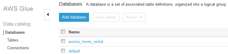
Hitting the checkbox on aurora_movie_rental, then clicking View Tables, we see our newly-catalogued tables in the next screenshot below. 

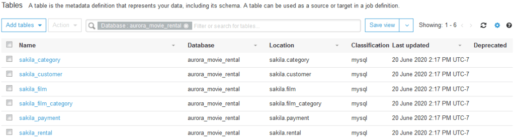
Notice a few things in the above screenshot

• Headers: Name of Tables, Classification, Last updated and Deprecated status.
• Database:  In the Glue Data Catalog, a database is no more than a logical grouping of tables.  In the search box, if the entered filter was removed, then tables from all databases would display.
• Location: At this point, these are still the data store’s RDBMS tables, and these paths are now available for subsequent Glue, Athena, Presto, or Redshift Spectrum querying.

Glue ETL: Jobs

Now that we’ve catalogued our tables in Aurora, our next step is to load them into the S3 data lake.  For that, we navigate in the Glue Console to Jobs / Create Job, and among the items we will enter, those that bear discussion (but not individual screenshots) include:

• (Job) Name, and script file name: movie_rental_customer_pyspark
• Type: Spark (vs. Python Shell).
• ETL Language (for Spark Type): I chose Python (PySpark) vs. Scala
• This job runs: ‘A proposed script generated by AWS Glue’
• Clicking ‘Security Config …job parameters (optional..?):
  • Worker Type: Chose Standard vs. a multi-node option
  • Maximum capacity (DPU’s): 
    • My choice is two DPU’s, currently the minimum setting.
    • A Glue DPU is short for Data Processing Unit.  One DPU cuirrently equates to four vCPU’s and 16 GB RAM.
    • So, my choice above allocates up to 8 vCPU’s, 32 GB RAM)
    • 10 DPU’s is the default, which means up to 40 vCPUs and 160 GB RAM.
    • The minimum run (think chargeable) Spark cycle here is 10 minutes, but AWS documentation indicates that cluster spin-up and spin-down time are not charged, only actual run-time.
    • Also of note, a small job may spin up less than this allowed maximum.
    • Still, in this context, these entries can dramatically effect both the run duration and the dollar cost. As such, to me they feel more mandatory than optional.
• Next, I selected Data Source: DB = aurora_movie_rental), table = customer
• Then, I chose ‘Create tables in your data target’
  • Data Store = Amazon S3
  • Format = Parquet
  • Target Path = s3://glue-dest-movie-rental/customer (via browse folder icon)
•  Next, we will map the source columns to target columns, per the screenshot below. Columns can be created, moved, or removed.

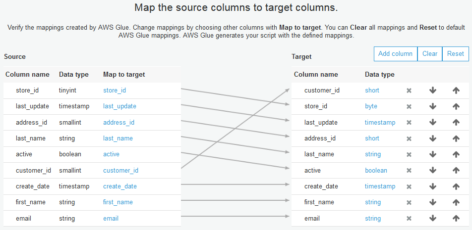
Because at this point, we are loading raw data into S3, we will not do any renaming, joins, or transformations now.

In the screenshot below, we see the Job’s PySpark Script and Flow Diagram

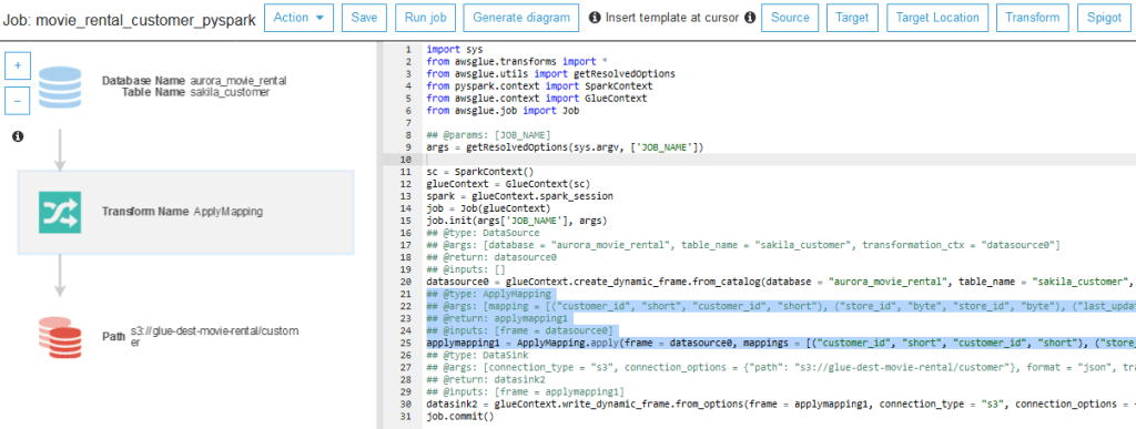
Takeaways from above screenshot:

• Ultra simple logic here: Read all records in all columns from the source and insert into the destination.
• Visual Highlighter: When the ApplyMapping Transform is highlighted in the left pane, it’s (generating) comments and code are highlighted on the right pane.
• As glue-generated PySpark script, the code lines lack carriage returns and extend far off the pane.
• Interestingly, this helpful diagram is generated exclusively by the green ## comments in the script. 
• With our cursor on a desired blank line in the script, clicking a button in the top right adds a generic comment-block and generic script for a number of available operations here, including built-in transforms, leaving us to then update the comments and the code with relevant details, after which we can click ‘Generate Diagram’, which will be as relevant and accurate as our comments.  
• If instead we either modify the script’s code without adding precisely formatted comments, or do not update the auto-generated generic comments from a template, the diagram will be out of sync with the script. A valid script will still run, but it will lack a diagram as a visual reference.

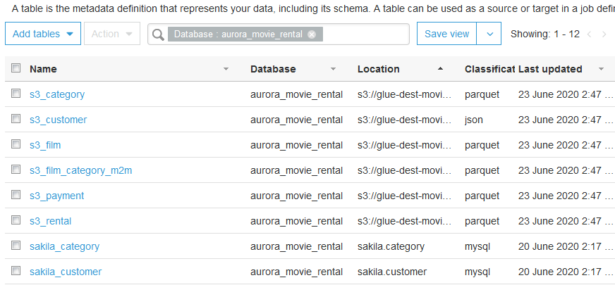
Now repeating the above process for our remaining tables, I have already built and run ETL jobs for them, and will now catalog the new objects in their new S3 location…

• New Crawler for Re-Cataloguing in S3: Run a new crawler, sourced this time from the new, S3 location for these tables, in order to catalog their properties from where they will be queried going forward.  Remember that the Glue Data Catalog is where not only Glue ETL jobs are run, but also where query engines like Athena, Presto, and Redshift Spectrum can query the actual data records in S3.  As such, this new crawler will catalog them with their new S3 path, their new classifications (ie. Parquet or JSON, not MySQL), and their partitions. 
• In the screenshot below, notice the newly catalogued tables w/ s3_ prefix (which I added), and their location (the exact S3 folder path), classification and last updated info. 

• Next, we build triggers to launch a given job within an overall GLUE ETL workflow to orchestrate dependencies among jobs and schedule the triggered job runs.

Glue ETL: Triggers and Workflow

Referring to the above screenshot, here are the notable items:

• Workflows having simple dependencies among jobs are easy to build with just bit of practice with this graph UI.
• Workflows always begin with a Trigger (depicted as a StopLight), which can be On Schedule, On Demand, or On Event.  Ours is on-demand, but AWS Lambda functions are commonly used to initiate Glue workflows.  A typical on-event trigger for a recurring Glue ETL workflows is the event wherein a new file arrives in an S3 bucket, wherein a Lambda function kicks off a Glue Workflow’s starting Trigger.
• Assuming that the jobs are configured with proper Spark cluster capacity, then running jobs in parallel as I’ve designed here means more efficient use of compute resources and a shorter overall run time.
• Note that some triggers ‘watch’ for completion of ‘ANY’ (one) job, while others watch for completion of ‘ALL’.

Glue ETL Job: Choice of PySpark or Python Shell for Code:

Obviously, dropping RDBMS tables into a data lake is often far from the end of required ETL.  So, we create new Glue ETL jobs, connecting to our newly catalogued S3 table, transform them and land them in S3, possible in another folder structure.  Doing this with Glue ETL offers us the following major choices:

Spark Jobs. When choosing PySpark (Python in the UI) we can use PySpark library’s DataFrames, SparkSQL, and other libraries.

Python Shell Jobs, including libraries like Pandas dataframes, iPython MagicSQL, or both.

Python Shell Downside: Because Glue does not currently offer auto-generated Python (hence the term ‘shell’), like it does provide for PySpark, running Python shell jobs requires hand-coding the Python script, including the importing of relevant Python libraries. Those Glue Development Endpoints, even though chargeable as long as they exist, are beginning to look good now. 

So, most of us will want to either instantiate a Glue Dev-Test Endpoint with Zeppelin Notebooks, or to connect another tool from our own machine, for example Jupyter notebooks, to the data source, write and validate the code there, then copy it to Glue’s Python shell script pane for the ETL job.

Python Shell Upside: Python shell jobs can run on either 1 DPU or .0625 (1/16 DPU), and have a shorter minimum run (and chargeable) period of 1 minute vs. PySpark’s 10 minutes, so for smaller or simpler processing jobs, it saves on Glue charges.

For AWS Glue pricing details, click here. With that, we will now get a quick look at Amazon Athena, which we will return to in more detailed future update.

Amazon Athena:

Athena is Amazon’s managed service in which we can query an S3 data lake, connected via a query-able data catalog, using ANSI SQL, and it is serverless, so as above, we do it without dealing with any RDBMS infrastructure, such as hardware, operating system, or database platform application.  Our detailed coverage of Athena in this blog entry is limited and primarily just to find and query the data we moved around using Glue.  Athena’s query engine is based on Apache Presto and the Apache Hive Metastore, and is purpose-built with the following features.  I will cover Quicksight, for data serverless data visualization and reporting, in a future post.

• Athena is serverless, unlike Presto, so we have no server machine to deal with.
• Limited insofar as Athena is aimed at querying S3 data lake, whereas as Presto queries a range of platforms.
• Athena offers workgroups, wherein we can segregate and manage access among members of business analysts teams outside of the data engineering team, and across the enterprise.
• Athena, being nicely integrated with S3, Glue, and Quicksight, is a crucial piece of the AWS serverless analytics proposition.  I was going to say “framework”, but AWS strongly favors a myriad of highly configurable services that they call “primitives”, not inflexible frameworks, for the sake of limitless adaptability to specific computing needs.  Of course, to fully leverage these myriad primitives, the learning curve is substantial, which is why, I hope, you’re still with me here. 
  • Together, dear reader, we got this! 
  • As an AWS framework builder, CloudFormation is intriguing for building-out entire purpose-specific application-stacks all at once, but is beyond the scope of this series.

Let’s navigate to the Athena console for a quick introduction. 

Because each AWS Account has just one Glue Data Catalog, connecting from Athena to Glue, once we arrive in the Athena Console, is as simple as selecting the AWS Region (top right of header bar) in which we built our Glue items, confirming our Data source, then selecting our database of interest.  In my case, it is ‘aurora_movie_rental’.

Notes:

• Our S3 tables are visible, but the MySQL tables, although catalogued in Glue, are not available to Athena.  If we were using Apache Presto (for instance within Amazon EMR) instead of Athena, and had set this same Glue Data Catalog as Presto’s default Hive metastore, then we would be able to  query tables catalogued there, via JDBC connectors from RDS, from Aurora, or from any connected on-premises instance of PostGres, MySQL, SQL Server, Oracle, Snowflake, and other database products.
  • Having said that, although Glue is able to run ETL jobs to-and-from these JDBC-connected databases, Glue Crawlers are not currently available for them, so the added benefit of crawler-based automatic cataloging is lost.
  • As such, an assessment of Athena and Presto should be done by teams up front. If you’ve already decided to standardize your data lake on S3, then Athena seems like a no brainer for an easy to use serverless query engine, with solid integration with Glue and, as we will cover later, with Quicksight for  data visualization and reporting. 

In the Athena query editor screenshot below, note that…

• We are in the query editor tab, which includes the following features
  • Clicking the ellipsis right of each table, ‘Preview Table’ creates a simple SQL query and runs it.
  • In the query window below, my ANSI SQL query has run and displays the results below.
  • Self-Service Features
    • After running a query, ‘Save as’ stores it in the ‘Saved Queries’ tab for future use.
    • ‘Create’ allows us to create a table or view in S3 from our query.
    • The ‘History’ tab at the top specifies when each query was run, it’s success, duration, volume of data scanned, and available actions during a subsequent browse, such as ‘download results’ (to Excel).
    • Workgroups is where we can segregate and secure the work of multiple team within Athena.

Much more to do in Athena, which I hope to return to in a future post.

Conclusion:  Serverless Data Engineering using AWS Glue with S3, Aurora, and Athena

To summarize what we have done here, we crawled an operational database, captured it’s metadata and query path in a queryable data catalog, loaded it into an S3 data lake, recatalogued it there, queried it with standard SQL through the data catalog using Athena, all without moving it out of the data lake, without dealing with the instantiation of any server infrastructure, and with the ability to easily shutdown any or all parts of this solution to eliminate ongoing costs. 

Self Service Business Intelligence on S3 Data Lake

With the data catalog and Athena’s workgroups, we can offer various analysts outside of the data engineering team the self-service capability to query either raw or curated data in an S3 data lake using standard SQL, which is a big advantage over traditional architectures in which we, the data engineering team, must extract the requested data, possible model it into a star schema, write and deploy more ETL code to load history and incremental updates.  

In my view, this serverless data engineering architecture is impressive, even without being coupled with additional serverless data querying, visualization and reporting, offering only what I have already demonstrated here. It is easy to envision that data analytics will increasingly be delivered from serverless environments going forward.

In a future posting, I will demonstrate, in no particular order, a more detailed use of Athena, Amazon Quicksight for serverless data visualization and reporting, and possible additional Glue ETL transformations.

If you benefited from reading this post, please respond by giving it your thumbs-up in the LinkedIn data feed, and feel free to add your comments or questions.

Thank you!